Roberto Vacca

Logistic Models: Forecasts based on Time Series -

By Roberto Vacca, - October 13, 2004

1 - Theory, equations, software The logistic substitution model considers separately each variable in a system context (e.g.: population (people [having certain features], cars, computers in use, installed kW, homes, transportation volumes, etc.) and determines for each the most probable equation governing the development process. The model, therefore, is agile and can be applied rapidly and easily expanded.
The model is based on the application of Volterra's equations. These were derived to analyze the development of biological populations and are represented by S shaped logistic curves. They depict accurately the mutual influences of two or more species competing in the same habitat for the same type of food. These equations describe accurately also the growth and the decline of populations of human products and artefacts. When historical data (time series) are available, the model determines the equation of the process and permits then to compute future developments.
If we call x the number of units belonging to a population, the equation is:

dx/dt = k x (N - x)


where the derivative is made with respect to time t. The solution is:

x = N/(1 + exp(A t + B))

where N is the asymptote or final constant measure of the population.

I developed the LOGI5000 software to fit an equation to a historical time series and compute the standard error of the measured data with respect to the equation. The fit can be considered adequate when the standard error is of the order of .01. When the standard error is much larger, we cannot affirm that the process can be described by means of a Volterra equation.
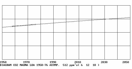
Volterra equations were used with great success in the past to describe development of a variable to fill an available ecological niche (biological populations, epidemics, CO2 in the atmosphere as described in the appendix). In some cases the fit is not satisfactory due to the presence of noise in the data.
The software used - and the mathematics on which it is founded - permit to assess the quality of the data used. Consequently the model provides also an indication of the credibility of the forecasts and projections it produces.

This procedure permits in many cases to forecast future levels of growth (or decline) with very high accuracy even 15 years in advance. The snag is that when you do produce a forecast like this you have no way of knowing you did. Example: the Italian car population. Until 1976 it could be forecast that the asymptote was 20 M vehicles, but in 1977 the curve switched to a slower one aiming at 35 M (on which we are now). This could not have been forecast in the early Seventies, but it was forecast as early as 1981. We could not be sure then that we had forecast accurately the future car park to 2002. We could say that this appeared as a very plausible outcome - which in this case proved to come true.

2 - An Example: Forecasting European Transportation
(Data from: "EU Transport in Figures 2000", European Union Directorate General for Energy and Transport, in cooperation with EUROSTAT)
We attempt here to produce transportation forecasts essentially based on time series of data from the same sector: mobility statistics, populations of vehicles, modal splits. These are considered not to depend on factors from different sectors: in a sense we consider here transportation variables as endogenous. This assumption happens to adhere to reality - for certain limited (but not necessarily too short) lengths of time and in certain contexts.

2.1 - Global mobility and modal splits
Passenger.kilometer data disaggregated by mode (a selection of which is given in Table 1) have been analysed by means of Volterra-Lotka equations using the LOGI5000 software. The results are depicted in Diagrams 1 to 3 showing the curves best fitting the experimental data.
For each diagram, the indication is given of the standard error in the fitting (which is quite low) and of the time constant, defined as the time for the variable to go from 10 to 90% of the asymptote.

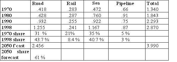
Table 1 - Passengers mobility EU15 (in G p.km)

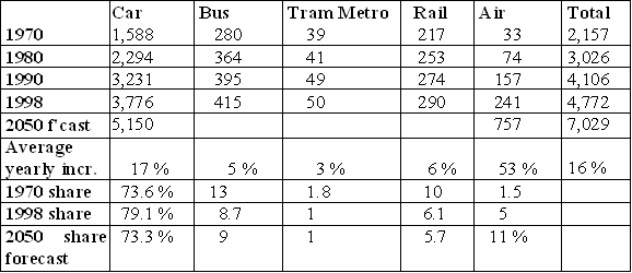
The decreasing shares of bus, tram/metro and rail travel are well known, as well as the increase in car travel and the faster increase of the share of air travel. The results of this analysis are shown in the bottom part of Table 1 and essentially they suggest the following conclusions:

Total passenger mobility tends to increase by about 50% in the next 50 years.

Car travel tends to grow in the next half century by 36% reaching 5,150 G p.km, but its share appears headed to decrease from79 to 73% (the same level as in 1970), due to the increase of air travel from 5% to 11%. This obviously applies to interurban mobility: urban travel appears headed towards continued dominance of the private car (see next section on Vehicle populations)

Present trends indicate that travel by bus, tram, metro and rail will continue to increase modestly, but their share will continue to decline. An obvious exception is represented by late comers to the construction of metro systems, like Rome

Cycling accounts for 5% of all trips and since these are normally shorter, the share does not even appear in Table 1. There are wide variations in share of total number of trips from high values in Netherlands (27%), Denmark (18%) and Sweden (13%) to very low ones in France (3%), UK (2%) and Spain (.7%).

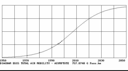
Diagram 1 - EU15 Total passenger mobility, asymptote 7,029 Gpass.km
Standard error = 2.7 E-03; Time constant = 78 years

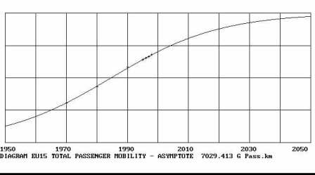
Diagram 2 - EU15 Total passenger mobility by car
(Standard Error = 3.9E-03; Time constant = 67 years)

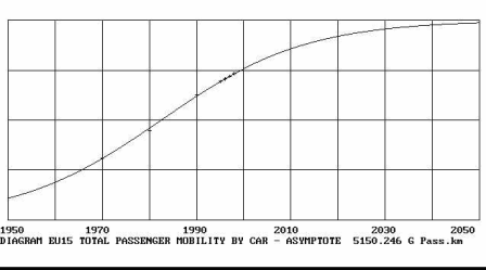
Diagram 3 - EU15 Total passenger mobility by air
Standard error = 1.1E-02; Time constant = 53 years

For goods transportation tonne.kilometer data disaggregated by mode (a selection of which is given in Table 2) have been analysed. However it was considered significant to use Volterra-Lotka equations only for goods transportation by road. The results are depicted in Diagram 4 showing the curve best fitting to the experimental data.

Table 2 - Goods mobility EU15 (in G t.km)


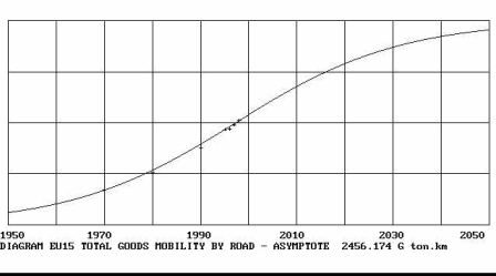
Here, again, a marked trend towards increasing predominance of road transport is visible. Half a century from now 61% of the 4 T ton.km moved in EU15 territory will go by truck and van.


Diagram 4 - EU15 total goods mobility by road
Standard error = 9E-03; Time constant = 75 years


2.2 -Vehicle populations
The forecasts presented above may be substantiated by analysing the growth of vehicle populations, the statistics of which are given in Table 3 for cars, busses and trucks.

Table 3 - EU15 Vehicle populations

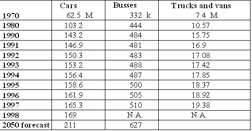
It was found possible to fit Volterra-Lotka equations only to the growth of cars and busses, as the data for trucks do not appear to follow this type of law. The curves obtained are represented in Diagrams 5 and 6. The car population appears plausibly to aim at a 25% increase, compatible with an increase of 36% in passenger.km.

Diagram 5 - EU15 total car population
Standard error = 1.67E-03; Time constant = 55 years


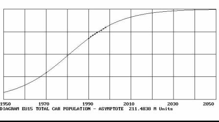
Here we have to note that often when a variable is nearing its asymptote, its values will present oscillations or hunting phenomena. Alternatively it often happens that before reaching the asymptote, a decline is initiated due to another variable substituting the former. A typical case is the sequence of substitutions of coal, by oil and then by gas. In the case of cars many signs indicate that in a decade or so internal combustion engines will be gradually replaced by electric motors fed by fuel cells (or by hydrogen stored in stable form as hydrides) or by hybrids. So the very definition of a car will have to be revised.

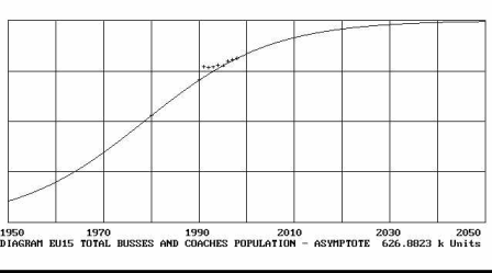
Diagram 6 - EU15 total busses and coaches population
Standard error = 8.8E-03; Time constant = 58 years


The growth of motorcycles has been of 18% from 1990 (8.6 M) to 1998 (10.1 M) and mopeds have decreased by 13% in the same period (from 14.9 M to 12.9 M). The decreasing share of rail transportation is confirmed by a decrease in stock. From 1970 to 1998: locomotives down to 55%, passenger coaches down to 77% and goods wagons down to 36%.