by Renato Croci
Aim of the present article is to provide an highlight about operating principles and techniques relevant to radar sensors. These sensor are currently employed not only in the 'classical' applications such as military or air traffic control, but are also widely used in scientific applications, i.e. airborne and spaceborne remote sensing, and onboard deep space probes.
Radar ( for "RAdio Detection And Ranging"), is a radio sensor, generally (but not always) operating in the microwave frequency range (> 1 GHz), and is an ACTIVE sensor. Here the word ACTIVE indicates that the sensor radiates energy (electromagnetic waves) toward the surrounding environment and extracts information about it through the analysis of the return echo.
Objects can be located:
Almost all current radars belong to the class called "monostatic", i.e. the transmitter and receiver are located together in a single equipment: bistatic and multistatic radars, on the other side, are those having the transmitter and one (ore more) receivers located in different places.
By the way, the first radar experimented by Watson-Watt (1937) was bistatic, with transmitter and receiver located several hundreds of meters away: the receiver detected a signal variation when an aircraft was flying above the area between the transmitter and the receiver, thus demonstrating the feasibility of radio detection of flying objects.
Common radars are pulsed: the transmitted signal is a "short" (i.e., from tens of nanosecs to tens of microsecs) pulse of radiofrequency, repeated periodically. During the time between two transmit pulses, the radar switches to receive mode to collect the return echoes (normally, using the same antenna used for the transmission)
When discussing about the radar range, a distinction must be made between the non-ambiguous range and the real detection range.
The non-ambiguous range is (for a pulsed radar) related to the Pulse Repetition Frequency (PRF, = 1/PRI, Pulse Repetition Interval)
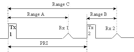
A typical radar timing is shown in fig.1: the two transmit pulses (Tx and Tx2) are divided by a time equal to the PRI. Rx1 is the echo from Tx1 reflected by a target placed at "Range A". Rx2 can be either the echo from Tx2 reflected by a target at "Range B" or from Tx1 reflected by a target at "Range C".
In the latter case the target is said to be at ambiguous range.
FIG. 1
The maximum non-ambiguous range is the one corresponding to the PRI:
Rna = PRI • c / 2
Note : it is anyway still possible to discriminate the real range of targets above the ambiguous range using staggered pulse repetition frequencies. The target at ambiguous range will then appear at different apparent ranges for each PRI, allowing a dedicated logic to solve the ambiguity and to extract the real range. This problem does not generally affects radars used, for instance, in spaceborne remote sensing: here the echoes are expected only in a well defined range window (corresponding to the range from the satellite to the illuminated points on the surface at minimum and maximum distance) and no echoes are expected between the radar and the Earth surface. This provides an a priori knowledge of the ambiguity, avoiding the need to use special techniques to solve it.
The non-ambiguous range provides only indication about the maximum range at which the target range information can be extracted unambiguously, and does not give any information about the maximum range at which a target can be detected. To derive the real detection range, the link budget shall be taken into account for the two paths radar-target and target-radar, together with the target characteristics. For the purpose of this introduction, the minimum Signal-to-Noise (S/N) ratio required for proper target detection will be considered as an input, and its determination will not be treated here.
NOTE: it is anyway important to remark that the radar detection is always a statistic process. The problem is to detect a signal within a gaussian noise: indipendently on how we can decide to position the decision threshold ("everything above the threshold is signal, everything below is noise") there is always a defined probability that: 1) the noise will exceed the threshold or 2) the signal + noise will be below the threshold (even if the signal itself would have been above the threshold). For a given S/N it is possible, changing the threshold, to reduce the probability of false alarm at the expense of the probability of detection. It is therefore uncorrect to say "this radar has a x km range on the target y" without adding "with 90% of probability of detection, and probability of false alarm 10^-6).
We will derive here the basics of the radar equation.
Let's have a transmitting antenna, isotropic, i.e. which radiates homogeneously in all directions. The transmitted power Pt, at a range R from the transmitter, is homogeneously spread over the surface of a sphere of radius R, with a power density:
![]()
Real antennas provide directivity: the antenna gain (G) is the measure of the antenna effectiveness in concentrating the radiated energy in the direction of interest. Then:
![]()
For a single-point target (a single-point target is a target having small dimensions compared to the angular and range resolution of the radar. For instance, for a typical search radar, a Boeing 747 is a single-point target), the target characteristics are accounted for through a parameter called cross-section (sigma, measured in m^2). A target having 1m^2 cross-section reflects toward the radar a power equivalent to all the power impinging on a surface of 1m^2 radiated isotropically (the physical area of the target may be smaller than its cross-section if it re-radiates preferentially toward the radar).
NOTE: for extended targets (like land or ocean surfaces) the target characteristics are accounted for through the reflectivity (sigma-0), a pure number having as reference a surface of the same area re-radiating isotropically all the impinging energy.
For the target-to-radar path, the same approach of the radar-target applies: the reflected power is spread on a spherical surface. The power density at the radar will then be:
![]()
The signal is collected by the receiving antenna proportionally to its effective area. If the same antenna is used for both transmit and receive, we can apply the formula relating the effective area to the gain:
![]()
The echo power returning at the receiver will then be:
![]()
The above formula does not take into account for simplicity the losses due to atmospheric attenuation and to the system non-idealities.
It must be noted that the received power decreases with the fourth power of the range: to double the radar range, the transmitting power must be increased by a factor of 16 ! (This applies for a single point target: if the target is a large surface, we shall take into account that the antenna beam becomes wider for increasing ranges, increasing the illuminated area and consequently the reflected power. Depending on the radar-surface geometry, the echo strength can be proportional to 1/R^3 or to 1/R^2.)
The echo signal shall be compared with the thermal noise. The noise equivalent power at the receiver input is given by:
Pn = kT B F
where :
k = Boltzmann's constant
T = receiver temperature (in degrees Kelvin)
B = Receiver noise bandwidth (can be roughly considered equal to the signal bandwidth)
F = Noise Figure, a term greater than 1, indicating how much the receiver is 'noisy' compared to the ideal case (F=1).
It is then possible to compute the S/N ratio.
It is important to remark that the receiver noise is proportionally to its bandwidth: this is also intuitive, being the thermal noise "white", i.e. homogeneously spread over the whole frequency spectrum. Increasing the receiver bandwidth will then increase the amount of noise energy developed inside the receiver. It is therefore important to keep the receiver bandwidth narrow, at the minimum level allowed by the need to provide proper amplification of the signal. For a simple pulse on a carrier, the optimum bandwidth is about B = 1/T (T = pulse length).
From a range point of view, it is therefore convenient, for the same peak power, to increase the pulse width (and therefore, its energy). Unfortunately, this requirement is in conflict with the range resolution requirement, as discussed later.
As a general rule, applicable to any radar waveform, it is possible to show that the range performance is relate only to the pulse energy, i.e. to the P x T product, at the condition that the receiver uses an "optimum" filter (called matched filter), having a frequency response complex conjugate of the signal spectrum (i.e., same amplitude response of the signal spectrum, and opposite phase response).
For a conventional radar, the angular resolution is equal to the aperture of the antenna beam, which, in turn, is related to the antenna linear dimension and to the signal wavelenght. For an antenna having linear dimension l, and for an operating wavelenght lambda, the beam aperture (in radiants) can be approximated by the formula:
![]()
The use of higher operating frequencies (shorter wavelenght) allows then to use smaller antennas for the same angular resolution.
Concerning the range resolution, it is possible to discriminate between separate echoes only if the difference in their delays is greater than the pulse width T. The range resolution is then T c/2.
The most straightforward way to improve the range resolution is then to use shorter pulses, i.e. larger pulse bandwidths (it can be demonstrated that the information content - the range resolution in our case - is proportional to the signal bandwidth): the drawback is that in this way the pulse energy is also reduced, degrading the performance in range if the other parameters are left unchanged.
The above constraints create severe problems in the design of high resolution radars: the transmitter technological limitations affects more the peak power than the average power or the energy of the single pulse. In other words, it is much easier to develop a transmitter capable of 2kW peak for 10 microsec than one providing 20kW peak for 1 microsec, even if the pulse energy is the same in both cases.
In order to achieve the advantage of both the "wide bandwidth" pulses in term of range resolution, and the use of "long" pulses with limited peak power, a technique called pulse coding is often used. In this technique, a form of modulation is superimposed to the long pulse, increasing its bandwidth. This modulation allows to discriminate between two pulses even if they are partially overlapped.
The range resolution of such a system can be approximated as T'=1/B (for an unmodulated pulse of duration T and bandwidth 1/T, it reduces to T'=T).
The two types of modulation most widely used in radar systems are the so-called chirp and the Barker Code: the former is a linear frequency modulation, the latter is a discrete (bi-phase) phase modulation.
In the receiver, the return signal is correlated with a stored replica of the transmit signal. For the chirp, it can be done applying the signal (normally in the Intermediate Frequency section of the receiver) to a dispersive delay line (i.e., having a delay which is linear function of the frequency), in order to concentrate all the pulse energy in a pulse shorter than the original one. It is also possible, taking advantage of the modern digital signal processing techniques, to perform, after analog-to-digital conversion, the convolution of the echo with a ideal single-point-target response (this is normally performed in the frequency domain, following a Fast Furier Transform of the signal, to improve the computational efficiency).
For the Barker Code, tapped delay lines with a summing/weigthing network are generally used. They can be implemented both in digital or in analog form (at intermediate frequency) using a (non-dispersive) delay line.
Many radars use the Doppler effect to extract information on targets radial velocity (almost all radars designed to detect aerial targets use the doppler effect to discriminate moving objects from the undesired fixed echoes).
A signal having wavelenght lambda is received by an observer in relative motion at radial velocity v with respect to the source as having a frequency shifted by an amount v/lambda from the transmitted frequency.
In the case of a radar, this effect occurs twice, on the radar-target and target-radar paths: the total Doppler shift is then:
![]()
At the normal radar frequencies, and for relative speeds in the order of tens or few hundreds m/sec (typical of aircrafts), the doppler shift is in the kHz range, the same order of magnitude of the PRF, and a period much shorter than the pulse width. This makes impossible to discriminate the frequency shift within the pulse.
All radars exploiting the doppler information use the same reference oscillators (characterised by high short-term frequency stability) in both the transmit and receive chains (see fig. 2). The local oscillator LO1 is the same for both chains. The received signal, instead of being demodulated using an envelope detector, is compared (normally using two channel having a 90 deg relative phase shift to extract the sin and cosin components of the signal) with the transmission reference frequency LO2 - the same used to generate the intermediate frequency transmit pulse - in a phase detector (a balanced mixer characterised by low offset voltage). The amplitude of the detected signal is proportional not only to the input signal amplitude, but also to the relative phase between the received signal and the reference (having used the same oscillators for both transmit and receive, the remaining frequency at the output is just the one due to the doppler shift).
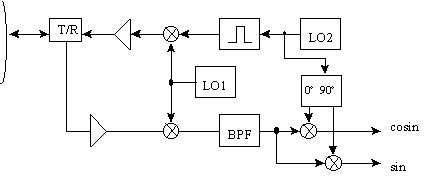
FIG 2
A return echo from a fixed target will have a zero doppler shift, and then a constant phase: all the return pulses from it will have the same amplitude after demodulation. If there is a doppler shift, the phase will change from pulse to pulse, and the amplitude of the demodulated signal will also change.
Using a two channels, sin-cosin demodulator, it is possible to unambiguously recover the phase of the return echo.
In other words, it is like as the envelope of the doppler frequency is sampled at the pulse repetition frequency. This is shown in fig. 3, which depicts the echoes of the same target in different PRIs at the output of the phase detector, together with the envelope of the doppler frequency. According to the sampling theorem, to avoid ambiguities in the measurement of the doppler frequency, the PRF must be, at least, twice the doppler frequency. This calls for the use of high PRFs, in conflict with the unambiguous range requirement discussed above. Ambiguities resolution techniques using staggered PRFs partially allow to conciliate this two requirements. (It must also be noted that, in many cases, the doppler ambiguity is not of concern, being the doppler shift used only to discriminate - and to cancel - all targets below a certain doppler shift, i.e. the fixed targets. For these systems, the only problem related to the doppler ambiguity occours when a target has a doppler shift which is an integer multiple of the PRF: it will be detected as a constant amplitude - zero doppler - return and then cancelled like a fixed echo.)
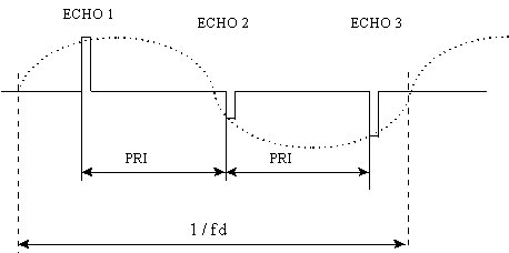
FIG 3
Where an accurate measurement of the doppler frequency is needed, continuous wave (CW) radars are used. Such radars do not provide any information about target range. Radars of this class, but with a moderate range resolution capability thanks to a frequency modulation of the signal carrier (FM-CW radars) are used for special applications (illuminating radars for missile guidance).
Last updated